Privacy cost estimation

This document is really just a proof of concept, but the basic idea is simple. I want to see how much data I can extract from a surveys on the cost of CCPA and GDPR from TrustArc. You can find details of that survey here.

library(MASS)
library(fitdistrplus) 
library(ggplot2)

So as a first matter, a range for the number of firms needs to be established. The Small Business Administration and go their data on the number of firms within this range. According to 2014 data, the total number of firms above 500 employees is 20,423. So, I set my total N as this.

N <- 20423 

Since I don’t have data on the relationship between company size and compliance cost, we are assuming that all firms could randomly assigned a compliance value. Of course, firm size is related to cost, so this assumption isn’t likely to hold in the real world, but work with me on it. Thus, we will be sampling N as a random uniform distribution from 0 to 1. The variable to store the samples from the mixture distribution is defined as dist_samples.

D <- runif(N)
dist_samples <- rep(NA,N)

Then we can take the data from the TrustArc survey, which is located on page 8, and sample it, using this method.

for(i in 1:N){
  if(D[i]<.03){
    dist_samples[i] = 0
  }else if(D[i]<.29){
    dist_samples[i] = runif(1, min = 0, max = 100)
  }else if(D[i]<.61){
    dist_samples[i] = runif(1, min = 100, max = 500)
  }else if(D[i]<.81){
    dist_samples[i] = runif(1, min = 500, max = 1000)
  }else if(D[i]<.96){
    dist_samples[i] = runif(1, min = 1000, max = 5000)
  }else{
    dist_samples[i] = 5000
  }
}

Next, plot the density of the random samples.

plot(density(dist_samples),main="Density Estimate of the Mixture Model", xlab="Compliance Cost in $1000s")

Naturally, we want to sum up all of these estimates, so let’s do that now.

sum(dist_samples)
## [1] 18316305

There we have it, an estimate for companies over 500 employees: $18,540,426,000. That’s massive, but understandable because we ran a uniform sample for all companies, which again, just won’t hold in the real world because we know there is a relationship between compliance cost and size.

Now this is only one estimate, so, let’s run 10,000 tests of this method.

estimate_samples <- rep(NA,10000)

for(s in 1:10000){
  N <- 20423 
  D <- runif(N)
  dist_samples <- rep(NA,N)

for(i in 1:N){
  if(D[i]<.03){
    dist_samples[i] = 0
  }else if(D[i]<.29){
    dist_samples[i] = runif(1, min = 0, max = 100)
  }else if(D[i]<.61){
    dist_samples[i] = runif(1, min = 100, max = 500)
  }else if(D[i]<.81){
    dist_samples[i] = runif(1, min = 500, max = 1000)
  }else if(D[i]<.96){
    dist_samples[i] = runif(1, min = 1000, max = 5000)
  }else{
    dist_samples[i] = 5000
  }
}
  estimate_samples[s]<- sum(dist_samples)
}

Oooof, that calculation took a while. So what is the mean and SD?

mean(estimate_samples)
## [1] 18565962
sd(estimate_samples)
## [1] 195413.6

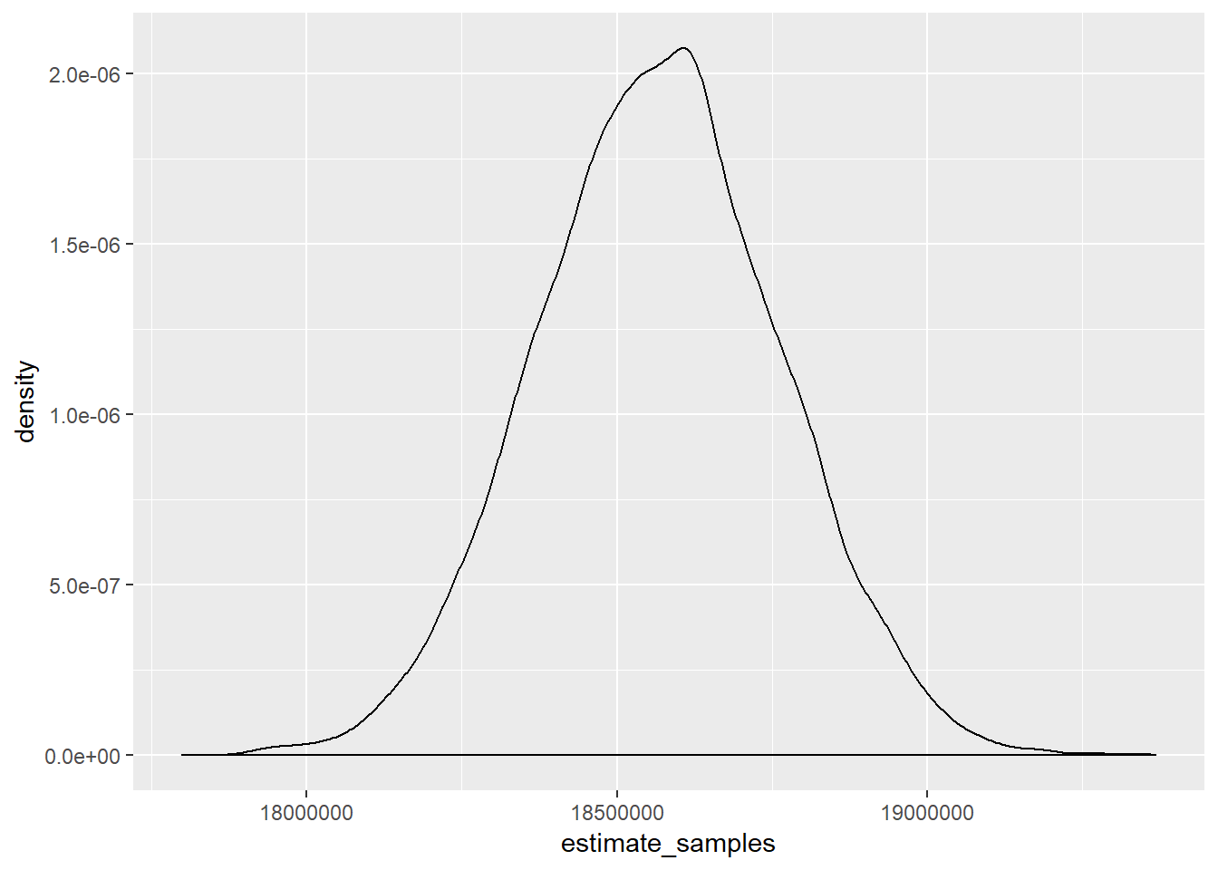
So the mean is $18,565,451,000. And what does the distribution look like?

dat<- data.frame(estimate_samples)
ggplot(dat, aes(x=estimate_samples)) + geom_density()